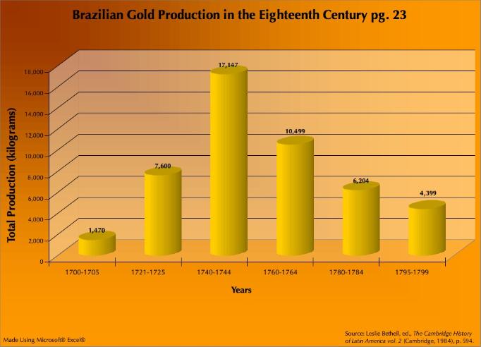
In this graph, it is most important to note the evidence of massive gold production that took place 1740-44, preceded and followed by a much smaller amount. The graphic representation of gold production shows why this period is called a gold “rush.”
Questions:
What group of people
typically ventured to the gold mines? Who actually did the mining?
Who made the most profit from this period of gold production?
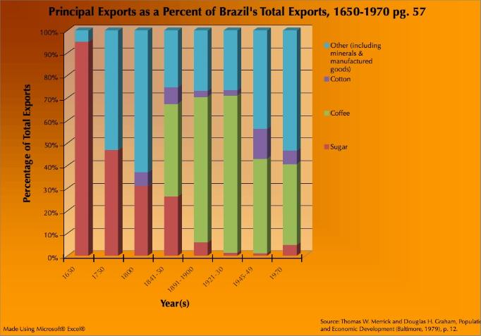
This graph illustrates the extent to which certain exports dominate Brazil’s total exports at different periods in the country’s history. Sugar and coffee both dominate at different points, sugar dropping dramatically after the colonial period. The percentage of “other” exports grows significantly during mineral deposit extractions (the gold rush of the mid-eighteenth century, for example) and during and after World War II, when Brazil began exporting raw materials like rubber and quartz in exchange for financial, military, and technical assistance from the United States. Finally, the story of coffee in this graph is particularly telling, especially in how coffee dominates 41.4% of exports, up from zero forty years earlier.
Questions:
What are the social and economic conditions that arise from the fact that in Brazil, almost always over half (if not almost all) its exports are raw materials?
Further, what conditions arise from the fact
that Brazil has frequently had one product that dominates its total exports?
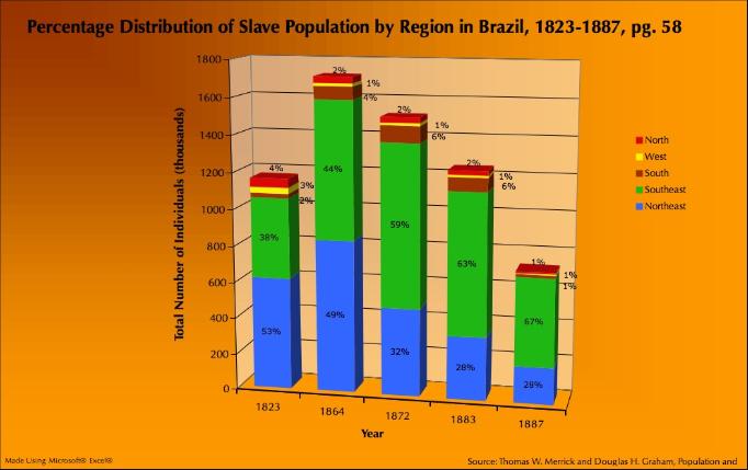
As coffee spread southward and production of this sector rose, there was an increased demand in slave labor to work the plantations. Just before the banning of the slave trade in 1850, there was a surge in slaves purchased given the knowledge that soon it would be illegal. After 1850, the southern providences looking for slave labor were forced to look toward domestic sources, especially in the North and Northeast. This exchange of labor resulted in a demographic shift southward. In this graph it is very easy to see the dropping percentage of slaves in the North and Northeast as the slave populations throughout the Southeast increased dramatically. The Southeast was the main receiver of slaves, however the southern region also increased its number of slaves mid-century before the numbers started dropping off once the slave trade was truly terminated.
Questions:
What impact did the demographic shift of slaves have upon the different regions of Brazil?
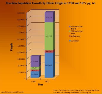 | 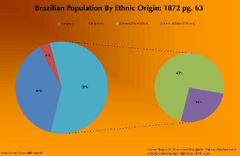 |
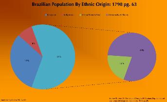 | Showing the Brazilian population by ethnic origin in two different kinds of graphs drives home two key points. First, while the population triples from 1798 to 1872, the raw numbers of indigenous and enslaved African/mixed peoples remains almost the same over that time. The European population increases, but most dramatic is the increase in free African/mixed peoples. Second, the two pie graphs show that while the total percentage of African/mixed peoples remains almost the same over the period, the sub-percentages of free and enslaved African/mixed peoples are completely reversed. Questions: From what you know about the history of Brazil before
1872, what explains the dramatic growth of the free African/mixed
population? Why does the indigenous population remain the same despite a
great increase in total population? |
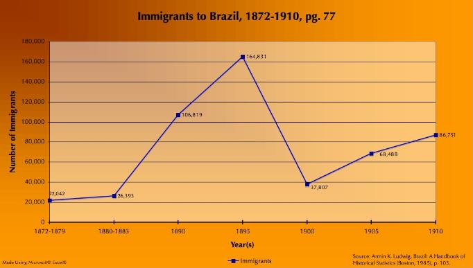
Once abolition took hold in Brazil, previous slave owners had to look elsewhere for their labor, a change that stimulated a remarkable surge in immigration. There were numerous reasons why planters failed to look toward national labor sources, including lack of faith in non-whites and the idea that immigrants would be easier to control. The majority of immigrants came from Europe, largely from Italy, Portugal and Spain, and went primarily to São Paulo and the South. These immigrants were fairly skilled and moved between different industries and national boundaries. In the graph, one can see the surge of immigrants after the abolition of slavery. As the country finally moved towards industrialization in the twentieth century, local and urban labor was more commonly used and the number of immigrants fell.
Questions:
What might the influx in immigrants as a source of labor say about the planter class of Brazil and the race and equality relations of that time period?
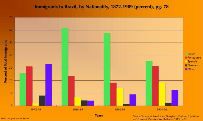
Corresponding to the previous graph, this graph shows the dominance and growth of the southern European immigrants, particularly the Italians. The growth and then fall in the numbers of these immigrants is in line with the trend seen in the previous graph.
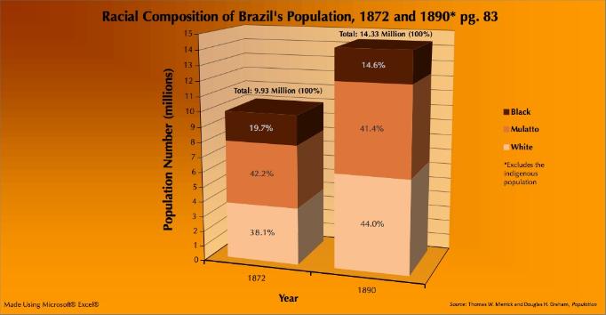
The important trend to witness in this graph is the increase in the number of white people within the population. This increase may be linked to the immigration occurring at the time. Many immigrants were coming from Europe and especially Italy. See the graphs from pages 77 and 78 for more information about immigration.
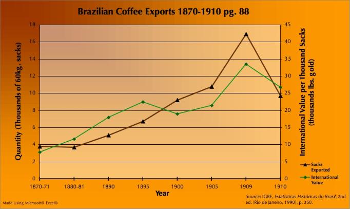
As this graph shows, the period between 1870 and 1909 was prosperous for Brazilian coffee producers. If one looks carefully one notices the sharp drop in values between 1909 and 1910 of the coffee crop and the corresponding drop in the number of sacks exported. This corresponds well to the graph from the table on pg. 57 outlining the central role that coffee took as Brazil’s main export during this time period.
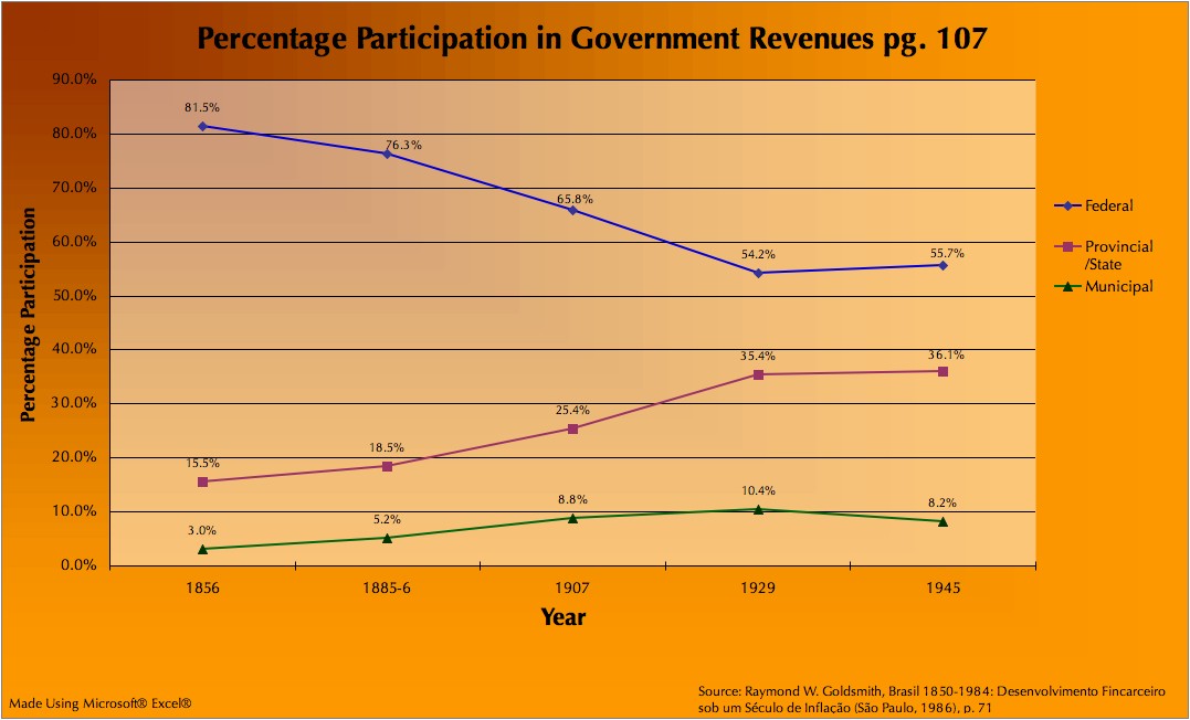
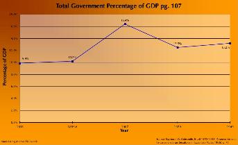 | The Constitution of 1891 allowed for much greater fragmentation of federal authority, giving states the power to control tariffs on goods crossing state borders, to negotiate international loans, and to manage the coffee trade and railway construction. In these charts, the decreasing share that the federal government contributed to overall government revenues is paired with the increasing share that state governments (and to some extent, municipal governments) contributed. Questions: While the 1891 Constitution allowed for decentralization of government powers, one of the graphs indicates that the total government percentage of Brazil’s GDP increased sharply at the time of the new Constitution, only to fall again after 1907. What could explain this change? |
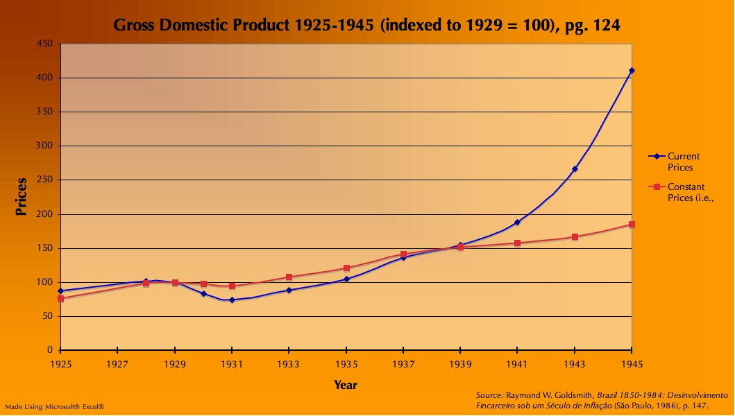
Brazil suffered a Depression after the crash of 1929, yet emerged from it much sooner than England or the United States, sustaining its recovery through World War II. At this time production was on the rise and with war stipulated technology and equipment from the United States, Brazil was able to modernize. Increased transportation and a turn toward domestic production instead of imports helped to accelerate Brazil’s growth. This graph clearly shows in both current and constant prices the initial depression in the GDP but then sustained growth throughout the Second World War period.
Questions:
What were the effects of World War II on the Brazilian economy?
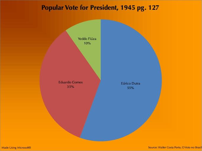
The 1945 election was the official end of Vargas’ dictatorship. The total votes cast in 1945 was three times the number cast in 1930, and the primary two candidates were both military officers: Eúrico Dutra, a general and candidate for the PSD, and Eduardo Gomes, air force brigadier and candidate for the UDN. While Gomes was a well-liked officer, he failed to gain enough popular support from the lower classes to win. Yeddo Fiúza, the Communist Party candidate, received a surprising 10% of the vote.
Questions:
What about the political and social situation in Brazil could explain why Fiúza, the Communist candidate, earned such a significant part of the total vote?
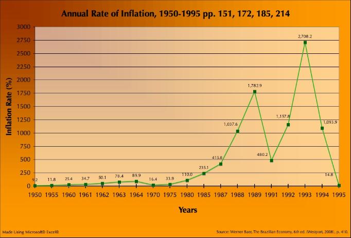
A careful look at this graph shows the story of the Brazilian economy’s inflation. The graph shows inflation rising steadily through the second half of the twentieth century, spiking in 1989 and 1993. The slow rise of inflation had many causes, much can be attributed to a series of presidents who ignored or worsened the country’s economy. The spikes in the late 1980s and early 1990s correlate with José Sarney’s presidency and the Cruzado Plan in 1988 and 1989, followed by continuing economic hardship and instability for several years until there was a sharp drop in inflation due to Fernando Henrique Cardoso’s Plano Real.
Questions:
What aspects of presidential policies and international factors in this period allowed inflation to continue to rise to such an extent it became part of the Brazilian norm?
Apart from economic hardships, what were other trends
in the 1980s and early 1990s that characterized such a difficult period in
Brazil’s recent history?
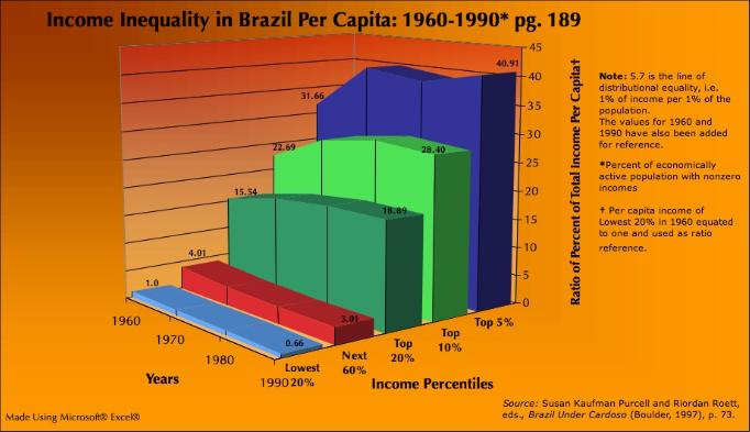
This graph is a little bit difficult to unpack, but once understood provides a stark viewpoint upon Brazil’s income inequality. Firstly, all ratios are scaled to the Lowest 20% of the population in 1960 which is used as our reference point, or 1. Income equality, meaning that 1% of the population takes home 1% of its income, is denoted on this graph by a ratio of 5.7. Therefore, a ratio below 5.7 means that the sector of the population is taking home less than its equal share of the income and a score above 5.7 means that the corresponding sector of the population is taking home more than its equal share of the income based complete distributional equality.
Looking at the trends in this graph, the main one is that the gap between the richest and poorest Brazilians has drastically increased since 1960. While the Lowest 20% has taken home less and less of the total national income the Top 20% has steadily increased its share. Separating this Top 20% into the Top 10% and the Top 5% only magnifies the difference. In 1990 the average household in the Top 5% of Brazilian wage earners took home more than sixty times the amount of the average household in the Bottom 20%. This is a substantial increase from 1960 when the difference was still large but only thirty-one to one.
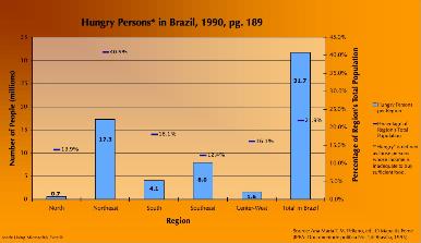 | Towards the end of the twentieth century there was an even greater gap forming between the rich and the poor. The economic boom of the 1970s increased the level of income inequality, but as always it varied greatly from region to region. This graph depicts the changing number of those deemed ‘hungry’ (people whose income was inadequate to allow for them to buy sufficient food). In 1990 in Brazil there were over 31 million people determined hungry and a majority of them were from the Northeast. Questions: From what you know about the different regions of Brazil, explain why the income inequality might be so related to regional characteristics. |